================ by Jawad Haider

02 - Numpy Operations¶

Copyright Qalmaqihir For more information, visit us at www.github.com/qalmaqihir/

1 NumPy Operations
1.1 Arithmetic
1.2 Universal Array Functions
1.3 Summary Statistics on Arrays
1.4 Axis Logic
2 Great Job! Thats the end of this part.

NumPy Operations¶

Arithmetic¶

You can easily perform array with array arithmetic, or scalar with array arithmetic. Let’s see some examples:

import numpy as np
arr = np.arange(0,10)
arr

array([0, 1, 2, 3, 4, 5, 6, 7, 8, 9])

arr + arr

array([ 0,  2,  4,  6,  8, 10, 12, 14, 16, 18])

arr * arr

array([ 0,  1,  4,  9, 16, 25, 36, 49, 64, 81])

arr - arr

array([0, 0, 0, 0, 0, 0, 0, 0, 0, 0])

# This will raise a Warning on division by zero, but not an error!
# It just fills the spot with nan
arr/arr

C:\Anaconda3\envs\tsa_course\lib\site-packages\ipykernel_launcher.py:3: RuntimeWarning: invalid value encountered in true_divide
  This is separate from the ipykernel package so we can avoid doing imports until

array([nan,  1.,  1.,  1.,  1.,  1.,  1.,  1.,  1.,  1.])

# Also a warning (but not an error) relating to infinity
1/arr

C:\Anaconda3\envs\tsa_course\lib\site-packages\ipykernel_launcher.py:2: RuntimeWarning: divide by zero encountered in true_divide


array([       inf, 1.        , 0.5       , 0.33333333, 0.25      ,
       0.2       , 0.16666667, 0.14285714, 0.125     , 0.11111111])

arr**3

array([  0,   1,   8,  27,  64, 125, 216, 343, 512, 729], dtype=int32)

Universal Array Functions¶

NumPy comes with many universal array functions, or ufuncs, which are essentially just mathematical operations that can be applied across the array.
Let’s show some common ones:

# Taking Square Roots
np.sqrt(arr)

array([0.        , 1.        , 1.41421356, 1.73205081, 2.        ,
       2.23606798, 2.44948974, 2.64575131, 2.82842712, 3.        ])

# Calculating exponential (e^)
np.exp(arr)

array([1.00000000e+00, 2.71828183e+00, 7.38905610e+00, 2.00855369e+01,
       5.45981500e+01, 1.48413159e+02, 4.03428793e+02, 1.09663316e+03,
       2.98095799e+03, 8.10308393e+03])

# Trigonometric Functions like sine
np.sin(arr)

array([ 0.        ,  0.84147098,  0.90929743,  0.14112001, -0.7568025 ,
       -0.95892427, -0.2794155 ,  0.6569866 ,  0.98935825,  0.41211849])

# Taking the Natural Logarithm
np.log(arr)

C:\Anaconda3\envs\tsa_course\lib\site-packages\ipykernel_launcher.py:2: RuntimeWarning: divide by zero encountered in log


array([      -inf, 0.        , 0.69314718, 1.09861229, 1.38629436,
       1.60943791, 1.79175947, 1.94591015, 2.07944154, 2.19722458])

Summary Statistics on Arrays¶

NumPy also offers common summary statistics like sum, mean and max. You would call these as methods on an array.

arr = np.arange(0,10)
arr

array([0, 1, 2, 3, 4, 5, 6, 7, 8, 9])

arr.sum()

arr.mean()

4.5

arr.max()

Other summary statistics include:

arr.min() returns 0                   minimum
arr.var() returns 8.25                variance
arr.std() returns 2.8722813232690143  standard deviation

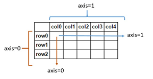
Axis Logic¶

When working with 2-dimensional arrays (matrices) we have to consider rows and columns. This becomes very important when we get to the section on pandas. In array terms, axis 0 (zero) is the vertical axis (rows), and axis 1 is the horizonal axis (columns). These values (0,1) correspond to the order in which arr.shape values are returned.

Let’s see how this affects our summary statistic calculations from above.

arr_2d = np.array([[1,2,3,4],[5,6,7,8],[9,10,11,12]])
arr_2d

array([[ 1,  2,  3,  4],
       [ 5,  6,  7,  8],
       [ 9, 10, 11, 12]])

arr_2d.sum(axis=0)

array([15, 18, 21, 24])

By passing in axis=0, we’re returning an array of sums along the vertical axis, essentially [(1+5+9), (2+6+10), (3+7+11), (4+8+12)]

arr_2d.shape

(3, 4)

This tells us that arr_2d has 3 rows and 4 columns.

In arr_2d.sum(axis=0) above, the first element in each row was summed, then the second element, and so forth.

So what should arr_2d.sum(axis=1) return?

# THINK ABOUT WHAT THIS WILL RETURN BEFORE RUNNING THE CELL!
arr_2d.sum(axis=1)

Great Job! Thats the end of this part.¶

Don't forget to give a star on github and follow for more curated Computer Science, Machine Learning materials